In parameter estimation techniques, several methods exist for estimating the distribution parameters in life data analysis. However, some of them are less efficient than Bayes’ method, despite its subjectivity to prior information other than data that can mislead subsequent inferences. Thus, the main objective of this study is to present optimal numerical iteration techniques, such as the Picard and the Runge-Kutta methods, which are more efficient than Bayes’ method. The proposed methods have been applied to the inverse Weibull distribution parameters and compared to the Bayes’ method based on the informative gamma prior and the non-parametric kernel and characteristic priors, via an extensive Monte Carlo simulation study through the absolute average bias and the mean squared errors for the parameter estimators. The simulation results indicated that the Picard and Runge-Kutta methods provide better estimates and outperform the Bayes’ method based on the dual generalized progressive hybrid censoring data. Finally, it has been shown that the inverse Weibull distribution gives a good fit to new areas of dataset applications, such as flood data and reactor pump data. We have analyzed and illustrated the proposed methods using these datasets to confirm the simulation results.
| Published in | International Journal of Statistical Distributions and Applications (Volume 11, Issue 2) |
| DOI | 10.11648/j.ijsda.20251102.12 |
| Page(s) | 28-44 |
| Creative Commons |
This is an Open Access article, distributed under the terms of the Creative Commons Attribution 4.0 International License (http://creativecommons.org/licenses/by/4.0/), which permits unrestricted use, distribution and reproduction in any medium or format, provided the original work is properly cited. |
| Copyright |
Copyright © The Author(s), 2025. Published by Science Publishing Group |
Bayesian Estimation, Characteristic Prior, Informative Prior, Kernel Prior, Picard’s Method, Runge- Kutta Method
n | m | k |
|
| Picard Estimates | R-K Estimates | Bayes estimates | ||
|---|---|---|---|---|---|---|---|---|---|
Gamma Prior | Chara-Prior | Kernel Prior | |||||||
20 | 10 | 5 | 1 | 2 | 0.0977(0.0097) | 0.1134(0.0129) | 0.1831(0.0336) | 0.1517(0.0230) | 0.1735(0.0301) |
3 | 0.1115(0.0127) | 0.1076(0.0116) | 0.1966(0.0466) | 0.1512(0.0229) | 0.1670(0.0279) | ||||
2 | 2 | 0.1282(0.0164) | 0.3199(0.1041) | 0.3772(0.1426) | 0.3126(0.0977) | 0.3479(0.1211) | |||
3 | 0.1347(0.0182) | 0.2804(0.0795) | 0.4078(0.2459) | 0.3083(0.0951) | 0.3354(0.1125) | ||||
8 | 1 | 2 | 0.0977(0.0097) | 0.1133(0.0129) | 0.1832(0.0336) | 0.1517(0.0230) | 0.1735(0.0301) | ||
3 | 0.1113(0.0126) | 0.1078(0.0116) | 0.1996(0.0558) | 0.1512(0.0229) | 0.1670(0.0279) | ||||
2 | 2 | 0.1283(0.0165) | 0.3185(0.1031) | 0.3765(0.1420) | 0.3124(0.0976) | 0.3476(0.1209) | |||
3 | 0.1341(0.0180) | 0.2815(0.0800) | 0.4017(0.1744) | 0.3084(0.0951) | 0.3356(0.1126) | ||||
15 | 8 | 1 | 2 | 0.0962(0.0094) | 0.1179(0.0140) | 0.1724(0.0297) | 0.1521(0.0231) | 0.1694(0.0287) | |
3 | 0.1109(0.0125) | 0.1088(0.0118) | 0.1701(0.0290) | 0.1513(0.0229) | 0.1646(0.0271) | ||||
2 | 2 | 0.1236(0.0153) | 0.3165(0.1016) | 0.3461(0.1198) | 0.3123(0.0975) | 0.3383(0.1144) | |||
3 | 0.1291(0.0167) | 0.2800(0.0791) | 0.3333(0.1111) | 0.3082(0.0950) | 0.3280(0.1076) | ||||
11 | 1 | 2 | 0.0964(0.0094) | 0.1172(0.0138) | 0.1725(0.0298) | 0.1521(0.0231) | 0.1694(0.0287) | ||
3 | 0.1108(0.0125) | 0.1087(0.0118) | 0.1699(0.0289) | 0.1513(0.0229) | 0.1645(0.0271) | ||||
2 | 2 | 0.1238(0.0154) | 0.3143(0.1002) | 0.3457(0.1196) | 0.3120(0.0974) | 0.3380(0.1143) | |||
3 | 0.1291(0.0167) | 0.2801(0.0791) | 0.3334(0.1111) | 0.3083(0.0950) | 0.3280(0.1076) | ||||
40 | 20 | 10 | 1 | 2 | 0.0927(0.0087) | 0.1136(0.0129) | 0.1644(0.0270) | 0.1517(0.0230) | 0.1622(0.0263) |
3 | 0.1063(0.0114) | 0.1079(0.0116) | 0.1630(0.0266) | 0.1512(0.0228) | 0.1589(0.0252) | ||||
2 | 2 | 0.1233(0.0152) | 0.3121(0.0981) | 0.3329(0.1108) | 0.3117(0.0971) | 0.3281(0.1076) | |||
3 | 0.1292(0.0167) | 0.2775(0.0774) | 0.3250(0.1056) | 0.3078(0.0948) | 0.3202(0.1026) | ||||
15 | 1 | 2 | 0.0923(0.0086) | 0.1138(0.0130) | 0.1644(0.0270) | 0.1517(0.0230) | 0.1622(0.0263) | ||
3 | 0.1062(0.0114) | 0.1080(0.0117) | 0.1630(0.0266) | 0.1512(0.0229) | 0.1589(0.0252) | ||||
2 | 2 | 0.1233(0.0152) | 0.3113(0.0976) | 0.3327(0.1107) | 0.3116(0.0971) | 0.3280(0.1076) | |||
3 | 0.1290(0.0167) | 0.2776(0.0774) | 0.3250(0.1056) | 0.3079(0.0948) | 0.3203(0.1026) | ||||
30 | 15 | 1 | 2 | 0.0919(0.0085) | 0.1161(0.0135) | 0.1628(0.0265) | 0.1519(0.0231) | 0.1614(0.0260) | |
3 | 0.1070(0.0116) | 0.1092(0.0119) | 0.1612(0.0260) | 0.1513(0.0229) | 0.1585(0.0251) | ||||
2 | 2 | 0.1238(0.0154) | 0.3217(0.1042) | 0.3314(0.1099) | 0.3127(0.0978) | 0.3278(0.1075) | |||
3 | 0.1302(0.0170) | 0.2856(0.0819) | 0.3236(0.1047) | 0.3087(0.0953) | 0.3203(0.1026) | ||||
23 | 1 | 2 | 0.0911(0.0084) | 0.1176(0.0139) | 0.1623(0.0264) | 0.1521(0.0231) | 0.1611(0.0260) | ||
3 | 0.1072(0.0116) | 0.1108(0.0123) | 0.1609(0.0259) | 0.1514(0.0229) | 0.1585(0.0251) | ||||
2 | 2 | 0.1258(0.0158) | 0.3296(0.1093) | 0.3319(0.1102) | 0.3135(0.0983) | 0.3283(0.1078) | |||
3 | 0.1328(0.0177) | 0.2943(0.0870) | 0.3249(0.1056) | 0.3096(0.0959) | 0.3214(0.1033) | ||||
60 | 30 | 15 | 1 | 2 | 0.0920(0.0085) | 0.1135(0.0129) | 0.1605(0.0258) | 0.1517(0.0230) | 0.1591(0.0253) |
3 | 0.1048(0.0111) | 0.1080(0.0117) | 0.1598(0.0255) | 0.1512(0.0228) | 0.1567(0.0246) | ||||
2 | 2 | 0.1241(0.0154) | 0.3143(0.0992) | 0.3275(0.1072) | 0.3119(0.0973) | 0.3241(0.1050) | |||
3 | 0.1301(0.0169) | 0.2782(0.0776) | 0.3212(0.1032) | 0.3078(0.0948) | 0.3171(0.1006) | ||||
23 | 1 | 2 | 0.0919(0.0085) | 0.1136(0.0129) | 0.1605(0.0258) | 0.1517(0.0230) | 0.1591(0.0253) | ||
3 | 0.1046(0.0110) | 0.1081(0.0117) | 0.1599(0.0256) | 0.1512(0.0228) | 0.1567(0.0246) | ||||
2 | 2 | 0.1240(0.0154) | 0.3150(0.0997) | 0.3276(0.1073) | 0.3120(0.0973) | 0.3242(0.1051) | |||
3 | 0.1298(0.0169) | 0.2789(0.0780) | 0.3213(0.1033) | 0.3079(0.0948) | 0.3172(0.1006) | ||||
45 | 23 | 1 | 2 | 0.0908(0.0083) | 0.1165(0.0136) | 0.1589(0.0252) | 0.1519(0.0231) | 0.1582(0.0250) | |
3 | 0.1050(0.0111) | 0.1089(0.0119) | 0.1577(0.0249) | 0.1512(0.0229) | 0.1561(0.0244) | ||||
2 | 2 | 0.1225(0.0150) | 0.3158(0.1001) | 0.3242(0.1051) | 0.3120(0.0974) | 0.3223(0.1039) | |||
3 | 0.1283(0.0165) | 0.2810(0.0792) | 0.3174(0.1007) | 0.3081(0.0949) | 0.3158(0.0997) | ||||
34 | 1 | 2 | 0.0913(0.0084) | 0.1167(0.0136) | 0.1590(0.0253) | 0.1520(0.0231) | 0.1582(0.0250) | ||
3 | 0.1062(0.0114) | 0.1101(0.0121) | 0.1577(0.0249) | 0.1513(0.0229) | 0.1562(0.0244) | ||||
2 | 2 | 0.1251(0.0157) | 0.3294(0.1090) | 0.3261(0.1063) | 0.3135(0.0983) | 0.3240(0.1050) | |||
3 | 0.1318(0.0174) | 0.2919(0.0855) | 0.3197(0.1022) | 0.3093(0.0957) | 0.3175(0.1008) | ||||
n | m | k |
|
| Picard Estimates | R-K Estimates | Bayes estimates | ||
|---|---|---|---|---|---|---|---|---|---|
Gamma Prior | Chara-Prior | Kernel Prior | |||||||
20 | 10 | 5 | 1 | 2 | 0.0811(0.0067) | 0.1046(0.0109) | 0.1455(0.0776) | 0.1509(0.0228) | 0.2567(0.1102) |
3 | 0.0913(0.0086) | 0.1025(0.0105) | 0.1378(0.0191) | 0.1506(0.0227) | 0.1887(0.0376) | ||||
2 | 2 | 0.1135(0.0129) | 0.2519(0.0639) | 0.5169(0.6370) | 0.3054(0.0933) | 0.3512(0.1235) | |||
3 | 0.1199(0.0145) | 0.2379(0.0569) | 0.4438(0.6048) | 0.3039(0.0924) | 0.3360(0.1129) | ||||
8 | 1 | 2 | 0.0951(0.0092) | 0.1095(0.0120) | 0.1991(0.0402) | 0.1514(0.0229) | 0.1761(0.0310) | ||
3 | 0.1082(0.0120) | 0.1053(0.0111) | 0.2479(0.1897) | 0.1510(0.0228) | 0.1678(0.0282) | ||||
2 | 2 | 0.1276(0.0163) | 0.2618(0.0689) | 0.3723(0.1390) | 0.3064(0.0939) | 0.3411(0.1164) | |||
3 | 0.1318(0.0174) | 0.2518(0.0636) | 0.4076(0.1972) | 0.3053(0.0932) | 0.3325(0.1105) | ||||
15 | 8 | 1 | 2 | 0.0952(0.0092) | 0.1092(0.0119) | 0.2024(0.0457) | 0.1513(0.0229) | 0.1760(0.0310) | |
3 | 0.1083(0.0120) | 0.1053(0.0111) | 0.2631(0.5345) | 0.1510(0.0228) | 0.1678(0.0282) | ||||
2 | 2 | 0.1281(0.0164) | 0.2601(0.0679) | 0.3709(0.1380) | 0.3062(0.0937) | 0.3406(0.1160) | |||
3 | 0.1318(0.0174) | 0.2517(0.0636) | 0.4302(0.3520) | 0.3053(0.0932) | 0.3324(0.1105) | ||||
11 | 1 | 2 | 0.1023(0.0105) | 0.1131(0.0128) | 0.1793(0.0322) | 0.1517(0.0230) | 0.1719(0.0296) | ||
3 | 0.1127(0.0129) | 0.1088(0.0119) | 0.1837(0.0339) | 0.1513(0.0229) | 0.1666(0.0278) | ||||
2 | 2 | 0.1415(0.0201) | 0.2692(0.0728) | 0.3525(0.1243) | 0.3071(0.0943) | 0.3362(0.1131) | |||
3 | 0.1454(0.0212) | 0.2614(0.0686) | 0.3550(0.1262) | 0.3063(0.0938) | 0.3302(0.1090) | ||||
40 | 20 | 10 | 1 | 2 | 0.0767(0.0059) | 0.1040(0.0108) | 0.1361(0.0188) | 0.1508(0.0227) | 0.2348(0.2390) |
3 | 0.0845(0.0072) | 0.1023(0.0105) | 0.1454(0.0211) | 0.1505(0.0227) | 0.2313(0.2259) | ||||
2 | 2 | 0.1129(0.0128) | 0.2485(0.0619) | 0.3933(0.1935) | 0.3050(0.0930) | 0.3323(0.1105) | |||
3 | 0.1176(0.0139) | 0.2382(0.0568) | 0.3995(0.3506) | 0.3039(0.0924) | 0.3233(0.1046) | ||||
15 | 1 | 2 | 0.0905(0.0082) | 0.1088(0.0118) | 0.1760(0.0312) | 0.1513(0.0229) | 0.1659(0.0275) | ||
3 | 0.1028(0.0107) | 0.1050(0.0110) | 0.2137(0.3842) | 0.1509(0.0228) | 0.1607(0.0258) | ||||
2 | 2 | 0.1269(0.0161) | 0.2547(0.0650) | 0.3385(0.1146) | 0.3056(0.0934) | 0.3259(0.1062) | |||
3 | 0.1305(0.0171) | 0.2471(0.0611) | 0.3528(0.1304) | 0.3048(0.0929) | 0.3208(0.1029) | ||||
30 | 15 | 1 | 2 | 0.0903(0.0082) | 0.1090(0.0119) | 0.1759(0.0311) | 0.1513(0.0229) | 0.1658(0.0275) | |
3 | 0.1033(0.0108) | 0.1049(0.0110) | 0.2065(0.0731) | 0.1509(0.0228) | 0.1606(0.0258) | ||||
2 | 2 | 0.1265(0.0160) | 0.2559(0.0656) | 0.3393(0.1152) | 0.3057(0.0935) | 0.3262(0.1064) | |||
3 | 0.1317(0.0174) | 0.2450(0.0601) | 0.3460(0.1206) | 0.3046(0.0928) | 0.3203(0.1026) | ||||
23 | 1 | 2 | 0.1099(0.0121) | 0.1117(0.0125) | 0.1638(0.0268) | 0.1516(0.0230) | 0.1615(0.0261) | ||
3 | 0.1146(0.0132) | 0.1089(0.0119) | 0.1638(0.0268) | 0.1513(0.0229) | 0.1591(0.0253) | ||||
2 | 2 | 0.1618(0.0262) | 0.2441(0.0596) | 0.3231(0.1044) | 0.3046(0.0928) | 0.3190(0.1018) | |||
3 | 0.1617(0.0262) | 0.2453(0.0602) | 0.3229(0.1043) | 0.3047(0.0928) | 0.3169(0.1004) | ||||
60 | 30 | 15 | 1 | 2 | 0.0829(0.0069) | 0.1045(0.0109) | 0.2109(0.1310) | 0.1509(0.0228) | 0.1672(0.0296) |
3 | 0.0943(0.0090) | 0.1025(0.0105) | 0.1937(0.2346) | 0.1506(0.0227) | 0.1587(0.0252) | ||||
2 | 2 | 0.1125(0.0127) | 0.2488(0.0620) | 0.3758(0.1572) | 0.3050(0.0930) | 0.3255(0.1060) | |||
3 | 0.1167(0.0136) | 0.2383(0.0569) | 0.3722(0.2935) | 0.3039(0.0923) | 0.3185(0.1015) | ||||
23 | 1 | 2 | 0.0897(0.0081) | 0.1087(0.0118) | 0.1751(0.0620) | 0.1513(0.0229) | 0.1618(0.0262) | ||
3 | 0.1015(0.0104) | 0.1051(0.0110) | 0.1873(0.0491) | 0.1509(0.0228) | 0.1578(0.0249) | ||||
2 | 2 | 0.1253(0.0157) | 0.2619(0.0687) | 0.3298(0.1088) | 0.3063(0.0938) | 0.3214(0.1033) | |||
3 | 0.1335(0.0178) | 0.2433(0.0592) | 0.3278(0.1075) | 0.3044(0.0927) | 0.3155(0.0995) | ||||
45 | 23 | 1 | 2 | 0.0895(0.0080) | 0.1089(0.0119) | 0.1651(0.0283) | 0.1513(0.0229) | 0.1619(0.0262) | |
3 | 0.1018(0.0104) | 0.1051(0.0110) | 0.1792(0.0356) | 0.1509(0.0228) | 0.1578(0.0249) | ||||
2 | 2 | 0.1251(0.0157) | 0.2619(0.0686) | 0.3297(0.1087) | 0.3063(0.0938) | 0.3214(0.1033) | |||
3 | 0.1329(0.0177) | 0.2444(0.0597) | 0.3289(0.1082) | 0.3045(0.0927) | 0.3157(0.0996) | ||||
34 | 1 | 2 | 0.1095(0.0120) | 0.1113(0.0124) | 0.1597(0.0255) | 0.1515(0.0230) | 0.1584(0.0251) | ||
3 | 0.1135(0.0129) | 0.1088(0.0118) | 0.1598(0.0255) | 0.1512(0.0229) | 0.1567(0.0246) | ||||
2 | 2 | 0.1675(0.0281) | 0.2394(0.0573) | 0.3163(0.1001) | 0.3042(0.0925) | 0.3142(0.0987) | |||
3 | 0.1652(0.0273) | 0.2416(0.0584) | 0.3161(0.0999) | 0.3044(0.0926) | 0.3128(0.0978) | ||||
n | m | k | Picard Estimates | R-K Estimates | Bayes estimates | ||||
|---|---|---|---|---|---|---|---|---|---|
Gamma prior | Chara-Prior | Kernel Prior | |||||||
20 | 10 | 5 | 1 | 2 | 0.0946(0.0090) | 0.1709(0.0296) | 0.4335(0.1883) | 0.2976(0.0885) | 0.3624(0.1313) |
3 | 0.1249(0.0156) | 0.2698(0.0732) | 0.7915(0.6591) | 0.4473(0.2001) | 0.5141(0.2643) | ||||
2 | 2 | 0.1022(0.0104) | 0.1072(0.0130) | 0.4309(0.1860) | 0.2915(0.0850) | 0.3536(0.1250) | |||
3 | 0.1364(0.0186) | 0.1820(0.0360) | 0.8130(0.8099) | 0.4391(0.1928) | 0.5032(0.2532) | ||||
8 | 1 | 2 | 0.0947(0.0090) | 0.1712(0.0296) | 0.4344(0.1890) | 0.2976(0.0886) | 0.3626(0.1315) | ||
3 | 0.1251(0.0157) | 0.2690(0.0727) | 0.7896(0.6701) | 0.4473(0.2001) | 0.5139(0.2641) | ||||
2 | 2 | 0.1021(0.0104) | 0.1083(0.0132) | 0.4301(0.1853) | 0.2916(0.0851) | 0.3536(0.1250) | |||
3 | 0.1366(0.0187) | 0.1788(0.0349) | 0.8161(0.7925) | 0.4389(0.1926) | 0.5031(0.2531) | ||||
15 | 8 | 1 | 2 | 0.0991(0.0099) | 0.1611(0.0264) | 0.3766(0.1420) | 0.2966(0.0880) | 0.3441(0.1184) | |
3 | 0.1303(0.0170) | 0.2654(0.0709) | 0.6113(0.3741) | 0.4469(0.1997) | 0.5018(0.2518) | ||||
2 | 2 | 0.1047(0.0110) | 0.1035(0.0122) | 0.3690(0.1362) | 0.2912(0.0848) | 0.3387(0.1147) | |||
3 | 0.1371(0.0188) | 0.1738(0.0329) | 0.5592(0.3127) | 0.4382(0.1921) | 0.4873(0.2375) | ||||
11 | 1 | 2 | 0.0988(0.0098) | 0.1630(0.0270) | 0.3782(0.1431) | 0.2968(0.0881) | 0.3448(0.1189) | ||
3 | 0.1304(0.0170) | 0.2656(0.0710) | 0.6095(0.3718) | 0.4469(0.1997) | 0.5016(0.2516) | ||||
2 | 2 | 0.1045(0.0109) | 0.1068(0.0127) | 0.3693(0.1364) | 0.2914(0.0849) | 0.3389(0.1149) | |||
3 | 0.1371(0.0188) | 0.1734(0.0327) | 0.5593(0.3129) | 0.4382(0.1921) | 0.4873(0.2375) | ||||
40 | 20 | 10 | 1 | 2 | 0.0976(0.0095) | 0.1690(0.0287) | 0.3560(0.1268) | 0.2973(0.0884) | 0.3336(0.1113) |
3 | 0.1288(0.0166) | 0.2674(0.0717) | 0.5606(0.3145) | 0.4470(0.1998) | 0.4882(0.2383) | ||||
2 | 2 | 0.1047(0.0110) | 0.1063(0.0121) | 0.3422(0.1171) | 0.2915(0.0850) | 0.3241(0.1051) | |||
3 | 0.1393(0.0194) | 0.1774(0.0332) | 0.5241(0.2747) | 0.4386(0.1923) | 0.4750(0.2256) | ||||
15 | 1 | 2 | 0.0978(0.0096) | 0.1683(0.0285) | 0.3558(0.1266) | 0.2973(0.0884) | 0.3335(0.1112) | ||
3 | 0.1289(0.0166) | 0.2669(0.0715) | 0.5598(0.3136) | 0.4470(0.1998) | 0.4880(0.2382) | ||||
2 | 2 | 0.1046(0.0110) | 0.1072(0.0123) | 0.3423(0.1172) | 0.2916(0.0850) | 0.3242(0.1051) | |||
3 | 0.1396(0.0195) | 0.1775(0.0329) | 0.5241(0.2747) | 0.4385(0.1923) | 0.4750(0.2256) | ||||
30 | 15 | 1 | 2 | 0.0998(0.0100) | 0.1628(0.0268) | 0.3437(0.1182) | 0.2967(0.0881) | 0.3277(0.1074) | |
3 | 0.1311(0.0172) | 0.2628(0.0693) | 0.5356(0.2869) | 0.4466(0.1995) | 0.4833(0.2336) | ||||
2 | 2 | 0.1044(0.0109) | 0.0997(0.0109) | 0.3333(0.1111) | 0.2909(0.0846) | 0.3197(0.1022) | |||
3 | 0.1393(0.0194) | 0.1689(0.0302) | 0.5076(0.2576) | 0.4378(0.1917) | 0.4705(0.2214) | ||||
23 | 1 | 2 | 0.1011(0.0103) | 0.1591(0.0256) | 0.3388(0.1148) | 0.2964(0.0878) | 0.3251(0.1057) | ||
3 | 0.1319(0.0174) | 0.2573(0.0665) | 0.5252(0.2759) | 0.4461(0.1990) | 0.4803(0.2307) | ||||
2 | 2 | 0.1035(0.0107) | 0.0978(0.0104) | 0.3295(0.1086) | 0.2906(0.0845) | 0.3175(0.1008) | |||
3 | 0.1401(0.0196) | 0.1634(0.0282) | 0.5029(0.2529) | 0.4373(0.1913) | 0.4684(0.2194) | ||||
60 | 30 | 15 | 1 | 2 | 0.0973(0.0095) | 0.1693(0.0288) | 0.3388(0.1148) | 0.2973(0.0884) | 0.3247(0.1054) |
3 | 0.1281(0.0164) | 0.2671(0.0715) | 0.5312(0.2823) | 0.4470(0.1998) | 0.4802(0.2306) | ||||
2 | 2 | 0.1042(0.0109) | 0.1063(0.0118) | 0.3284(0.1079) | 0.2915(0.0850) | 0.3163(0.1001) | |||
3 | 0.1400(0.0196) | 0.1797(0.0333) | 0.5049(0.2549) | 0.4387(0.1924) | 0.4682(0.2192) | ||||
23 | 1 | 2 | 0.0973(0.0095) | 0.1693(0.0288) | 0.3388(0.1148) | 0.2973(0.0884) | 0.3247(0.1054) | ||
3 | 0.1282(0.0164) | 0.2668(0.0713) | 0.5322(0.2834) | 0.4470(0.1998) | 0.4803(0.2307) | ||||
2 | 2 | 0.1042(0.0109) | 0.1056(0.0117) | 0.3285(0.1079) | 0.2914(0.0849) | 0.3163(0.1001) | |||
3 | 0.1402(0.0197) | 0.1782(0.0327) | 0.5051(0.2552) | 0.4385(0.1923) | 0.4681(0.2191) | ||||
45 | 23 | 1 | 2 | 0.1003(0.0101) | 0.1622(0.0265) | 0.3269(0.1068) | 0.2966(0.0880) | 0.3183(0.1013) | |
3 | 0.1316(0.0173) | 0.2639(0.0698) | 0.5082(0.2582) | 0.4466(0.1995) | 0.4753(0.2259) | ||||
2 | 2 | 0.1051(0.0111) | 0.1030(0.0112) | 0.3201(0.1025) | 0.2912(0.0848) | 0.3122(0.0975) | |||
3 | 0.1382(0.0191) | 0.1724(0.0308) | 0.4843(0.2346) | 0.4378(0.1917) | 0.4627(0.2141) | ||||
34 | 1 | 2 | 0.0998(0.0100) | 0.1620(0.0264) | 0.3266(0.1067) | 0.2966(0.0880) | 0.3181(0.1012) | ||
3 | 0.1315(0.0173) | 0.2601(0.0678) | 0.5027(0.2528) | 0.4463(0.1992) | 0.4733(0.2240) | ||||
2 | 2 | 0.1037(0.0108) | 0.0971(0.0100) | 0.3178(0.1010) | 0.2906(0.0844) | 0.3105(0.0964) | |||
3 | 0.1406(0.0198) | 0.1653(0.0284) | 0.4837(0.2340) | 0.4374(0.1913) | 0.4616(0.2131) | ||||
n | m | k | Picard Estimates | R-K Estimates | Bayes estimates | ||||
|---|---|---|---|---|---|---|---|---|---|
Gamma Prior | Chara-Prior | Kernel Prior | |||||||
20 | 10 | 5 | 1 | 2 | 0.0984(0.0098) | 0.1837(0.0339) | 0.6804(0.6774) | 0.2986(0.0892) | 0.6804(0.6774) |
3 | 0.1236(0.0153) | 0.2828(0.0802) | 0.7087(0.7177) | 0.4484(0.2010) | 0.7087(0.7177) | ||||
2 | 2 | 0.1124(0.0127) | 0.1406(0.0209) | 0.4113(0.1694) | 0.2946(0.0868) | 0.4113(0.1694) | |||
3 | 0.1349(0.0182) | 0.2133(0.0483) | 0.5449(0.2970) | 0.4419(0.1953) | 0.5449(0.2970) | ||||
8 | 1 | 2 | 0.0937(0.0088) | 0.1775(0.0317) | 0.3818(0.1458) | 0.2982(0.0889) | 0.3818(0.1458) | ||
3 | 0.1233(0.0152) | 0.2760(0.0765) | 0.5278(0.2786) | 0.4479(0.2006) | 0.5278(0.2786) | ||||
2 | 2 | 0.1024(0.0105) | 0.1531(0.0238) | 0.3696(0.1366) | 0.2958(0.0875) | 0.3696(0.1366) | |||
3 | 0.1347(0.0182) | 0.2186(0.0490) | 0.5160(0.2663) | 0.4425(0.1958) | 0.5160(0.2663) | ||||
15 | 8 | 1 | 2 | 0.0935(0.0088) | 0.1785(0.0320) | 0.3820(0.1459) | 0.2982(0.0890) | 0.3820(0.1459) | |
3 | 0.1233(0.0152) | 0.2762(0.0766) | 0.5275(0.2783) | 0.4479(0.2006) | 0.5275(0.2783) | ||||
2 | 2 | 0.1021(0.0104) | 0.1549(0.0243) | 0.3695(0.1365) | 0.2960(0.0876) | 0.3695(0.1365) | |||
3 | 0.1347(0.0182) | 0.2185(0.0489) | 0.5161(0.2664) | 0.4424(0.1958) | 0.5161(0.2664) | ||||
11 | 1 | 2 | 0.0937(0.0088) | 0.1745(0.0306) | 0.3568(0.1273) | 0.2979(0.0887) | 0.3568(0.1273) | ||
3 | 0.1258(0.0158) | 0.2667(0.0714) | 0.5087(0.2587) | 0.4471(0.1999) | 0.5087(0.2587) | ||||
2 | 2 | 0.0973(0.0095) | 0.1599(0.0258) | 0.3512(0.1234) | 0.2965(0.0879) | 0.3512(0.1234) | |||
3 | 0.1324(0.0175) | 0.2258(0.0516) | 0.5006(0.2506) | 0.4431(0.1964) | 0.5006(0.2506) | ||||
40 | 20 | 10 | 1 | 2 | 0.0994(0.0099) | 0.1850(0.0343) | 0.6416(0.5363) | 0.2987(0.0892) | 0.6416(0.4361) |
3 | 0.1238(0.0153) | 0.2830(0.0802) | 0.3526(0.1324) | 0.4482(0.2009) | 0.4253(0.3842) | ||||
2 | 2 | 0.1123(0.0126) | 0.1464(0.0219) | 0.3757(0.1413) | 0.2951(0.0871) | 0.3757(0.1413) | |||
3 | 0.1367(0.0187) | 0.2145(0.0473) | 0.5200(0.2705) | 0.4420(0.1953) | 0.5200(0.2705) | ||||
15 | 1 | 2 | 0.0945(0.0089) | 0.1784(0.0319) | 0.3579(0.1282) | 0.2982(0.0889) | 0.3579(0.1282) | ||
3 | 0.1233(0.0152) | 0.2770(0.0769) | 0.5082(0.2583) | 0.4480(0.2007) | 0.5082(0.2583) | ||||
2 | 2 | 0.1026(0.0105) | 0.1588(0.0253) | 0.3459(0.1196) | 0.2963(0.0878) | 0.3459(0.1196) | |||
3 | 0.1345(0.0181) | 0.2259(0.0514) | 0.4968(0.2468) | 0.4431(0.1963) | 0.4968(0.2468) | ||||
30 | 15 | 1 | 2 | 0.0946(0.0090) | 0.1778(0.0317) | 0.3571(0.1276) | 0.2982(0.0889) | 0.3571(0.1276) | |
3 | 0.1232(0.0152) | 0.2775(0.0772) | 0.5078(0.2579) | 0.4480(0.2007) | 0.5078(0.2579) | ||||
2 | 2 | 0.1028(0.0106) | 0.1574(0.0249) | 0.3461(0.1198) | 0.2962(0.0877) | 0.3461(0.1198) | |||
3 | 0.1338(0.0179) | 0.2306(0.0535) | 0.4967(0.2467) | 0.4435(0.1967) | 0.4967(0.2467) | ||||
23 | 1 | 2 | 0.0919(0.0084) | 0.1798(0.0324) | 0.3319(0.1101) | 0.2984(0.0890) | 0.3319(0.1101) | ||
3 | 0.1261(0.0159) | 0.2681(0.0720) | 0.4859(0.2361) | 0.4472(0.2000) | 0.4859(0.2361) | ||||
2 | 2 | 0.0929(0.0086) | 0.1812(0.0328) | 0.3282(0.1077) | 0.2985(0.0891) | 0.3282(0.1077) | |||
3 | 0.1284(0.0165) | 0.2563(0.0657) | 0.4811(0.2315) | 0.4460(0.1990) | 0.4811(0.2315) | ||||
60 | 30 | 15 | 1 | 2 | 0.0924(0.0086) | 0.1861(0.0347) | 0.3981(0.1956) | 0.2989(0.0893) | 0.3981(0.1956) |
3 | 0.1213(0.0147) | 0.2857(0.0817) | 0.5197(0.2702) | 0.4487(0.2013) | 0.5197(0.2702) | ||||
2 | 2 | 0.1126(0.0127) | 0.1462(0.0216) | 0.3602(0.1298) | 0.2951(0.0871) | 0.3602(0.1298) | |||
3 | 0.1375(0.0189) | 0.2144(0.0468) | 0.5087(0.2588) | 0.4419(0.1953) | 0.5087(0.2588) | ||||
23 | 1 | 2 | 0.0949(0.0090) | 0.1788(0.0320) | 0.3449(0.1191) | 0.2982(0.0889) | 0.3449(0.1191) | ||
3 | 0.1234(0.0152) | 0.2767(0.0767) | 0.4963(0.2463) | 0.4479(0.2006) | 0.4963(0.2463) | ||||
2 | 2 | 0.1034(0.0107) | 0.1518(0.0232) | 0.3336(0.1113) | 0.2957(0.0874) | 0.3336(0.1113) | |||
3 | 0.1330(0.0177) | 0.2362(0.0559) | 0.4854(0.2356) | 0.4440(0.1972) | 0.4854(0.2356) | ||||
45 | 23 | 1 | 2 | 0.0951(0.0091) | 0.1782(0.0318) | 0.3450(0.1193) | 0.2982(0.0889) | 0.3450(0.1193) | |
3 | 0.1234(0.0152) | 0.2769(0.0768) | 0.4961(0.2461) | 0.4479(0.2007) | 0.4961(0.2461) | ||||
2 | 2 | 0.1034(0.0107) | 0.1519(0.0232) | 0.3335(0.1112) | 0.2957(0.0874) | 0.3335(0.1112) | |||
3 | 0.1333(0.0178) | 0.2338(0.0548) | 0.4855(0.2357) | 0.4438(0.1970) | 0.4855(0.2357) | ||||
34 | 1 | 2 | 0.0918(0.0084) | 0.1805(0.0326) | 0.3234(0.1046) | 0.2984(0.0891) | 0.3234(0.1046) | ||
3 | 0.1260(0.0159) | 0.2683(0.0721) | 0.4780(0.2285) | 0.4472(0.2000) | 0.4780(0.2285) | ||||
2 | 2 | 0.0920(0.0085) | 0.1843(0.0340) | 0.3203(0.1026) | 0.2989(0.0893) | 0.3203(0.1026) | |||
3 | 0.1276(0.0163) | 0.2614(0.0683) | 0.4734(0.2241) | 0.4466(0.1994) | 0.4734(0.2241) | ||||
Data | The Tests | Calculated value | Critical value | The p-values | MLES | |
|---|---|---|---|---|---|---|
|
| |||||
Flood N=20 | K-S | 0.6976 | 0.8482 | 0.2138 | 4.3141 | 0.0119 |
A-D | 0.3104 | 0.7414 | 0.5899 | |||
CH2 | 3.5552 | 31.1109 | 0.3294 | |||
Reactor pumps N=23 | K-S | 0.4741 | 0.8528 | 0.8113 | 0.7832 | 0.4463 |
A-D | 0.3443 | 0.7472 | 0.4915 | |||
CH2 | 10.270 | 31.5744 | 0.1223 | |||
Sam. | T | Par. | Picard Estimate | R-K Estamite | Charact. Prior | Gamma Prior | Kernel Prior | |||||
|---|---|---|---|---|---|---|---|---|---|---|---|---|
Est. | MSE | Est. | MSE | Est. | MSE | Est. | MSE | Est. | MSE | |||
Data 4.1 N=20 | 0.25 |
| 4.1412 | 0.0298 | 3.9213 | 0.1539 | 3.6551 | 0.4337 | 3.5358 | 0.6051 | 3.6195 | 0.4819 |
| 0.0112 | 0.0001 | 0.0153 | 0.0002 | 0.0101 | 0.0003 | 0.0101 | 0.0003 | 0.0101 | 0.0003 | ||
0.65 |
| 4.1411 | 0.0297 | 3.3666 | 0.4192 | 3.6334 | 0.4629 | 3.4723 | 0.7079 | 3.5907 | 0.5227 | |
| 0.0110 | 0.0001 | 0.0133 | 0.0002 | 0.0099 | 0.00004 | 0.0098 | 0.0004 | 0.0099 | 0.0004 | ||
Data 4.2 N=23 | 0.15 |
| 0.7486 | 0.0012 | 0.7271 | 0.0031 | 0.6627 | 0.0145 | 0.6456 | 0.0189 | 0.6471 | 0.0185 |
| 0.3958 | 0.0025 | 0.4493 | 0.0011 | 0.3804 | 0.0043 | 0.3702 | 0.0058 | 0.3708 | 0.0057 | ||
5.0 |
| 0.7402 | 0.0018 | 0.7288 | 0.0029 | 0.6629 | 0.0144 | 0.6408 | 0.0203 | 0.6431 | 0.0196 | |
| 0.3922 | 0.0029 | 0.4446 | 0.0012 | 0.3798 | 0.0044 | 0.3661 | 0.0064 | 0.3671 | 0.0063 | ||
DGOS | The Dual Generalized Order Statistics |
GOS | Generalized Order Statistics |
IWD | Inverse Weibull Distribution |
MLE | Maximum Likelihood Estimators |
GPHCS | Generalized Progressive Hybrid Censoring Scheme |
DGPHCS | The Dual Generalized Progressive Hybrid Censoring Scheme |
AVB | The Absolute Average Bias |
MSE | The Root Mean Squared Error |
R-K | Runge-Kutta |
| [1] | Ahsanullah, M. (2000 a) Generalized order statistics from exponential distribution, J. Statist. Planning Inference, Vol. 85, P. 85–91. |
| [2] | Ahsanullah, M. (2000 b). The generalized order statistics from two parameter uniform distribution, Commun. Statist. -Theory Methods, Vol. 25, No. 10, P. 2311–2318. |
| [3] | Ahsanullah, M., Maswadah, M. and Seham, M. (2013). Kernel inference on the generalized gamma distribution based on generalized order statistics. J. Stat. Theory Appl. Vol. 12, pp. 152–172. |
| [4] | Burkschat M, Cramer E, Kamps U (2003) Dual generalized order statistics. Metron 61(1): 13–26. |
| [5] | Calabria, R. and Pulcini, G. (1989). Confidence limits for reliability and tolerance limits in the inverse Weibull distribution. Reliability Engineering and system safety, Vol. 24, P. 77-85. |
| [6] | Calabria, R. and Pulcini, G. (1990). On the maximum likelihood and least-squares estimation in the inverse Weibull distribution. Statistica applicata, Vol. 2, P. 53-66. |
| [7] | Calabria, R. and Pulcini, G. (1992). Bayes probability intervals in a load-strength model. Comm. In Statistics-Theory and Methods, Vol. 21, P. 3393-3405. |
| [8] | Calabria, R. and Pulcini, G. (1994). Bayes 2-Sample prediction for the Inverse Weibull Distribution. Commun. Statist. –Theory Meth., Vol. 23(6), P. 1811-1824. |
| [9] | Cho, Y., Sun, H., Lee, K. (2014). An estimation of the entropy for a Rayleigh distribution based on doubly generalized Type-II hybrid censored samples. Entropy, Vol. 16, P. 3655–3669. |
| [10] | Cho, Y., Sun, H., Lee, K. (2015 a). Exact likelihood inference for an exponential parameter under generalized progressive hybrid censoring scheme. Stat. Method, Vol. 23, P. 18–34. |
| [11] | Cho, Y., Sun, H. and Lee, K. (2015 b). Estimating the Entropy of a Weibull Distribution under Generalized Progressive Hybrid Censoring, Entropy, Vol. 17, P. 102-122; |
| [12] | Dumonceaux, R. and Antle, C. E. (1973): Discrimination between the Lognormal and Weibull distribution. Technometrics, 15, 923-926. |
| [13] | Erto, P. (1989). Genesis, properties and identification of the inverse Weibull lifetime model. Statistica Applicata, Vol. 2, P. 117-128. |
| [14] | Feuerverger, A. (1990). An efficiency result for the empirical characteristic function in stationary time series models. The Canadian Journal of Statistics. Vol. 18, P. 155-161. |
| [15] | Kamps U (1995) A concept of generalized order statistics. J Stat Plann Inference 48: 1–23. |
| [16] | Keller, A. Z. & Kamath, A. R. R. (1982). Alternative reliability models for mechanical systems. Paper presented at 3-rd international conference on Reliability and Maintainability, Toulouse, France. |
| [17] | Keller, A. Z., Giblin, M. T. and Farnworth, N. R. (1985). Reliability analysis of commercial vehicle engines Reliability Engineering, Vol. 10, P. 15-25. |
| [18] | Khan, M. S., Pasha, G. R. and Pasha, A. H. (2008 a). Theoretical analysis of inverse Weibull distribution. WSEAS Transaction on Mathematics. Vol. 7(2), P. 30-38. |
| [19] | Khan, M. S., Pasha, G. R. and Pasha, A. H. (2008 b). Fisher information matrix for the inverse Weibull distribution. International J. of. Math. Sci. & Eng. Appls. Vol. 2(3). P. 257-262. |
| [20] | Maswadah, M. (2003). Conditional Confidence Interval Estimation for the Inverse Weibull Distribution Based on Censored Generalized Order Statistics. J. Statist. Comput. Simul. Vol. 73, No. 12, P. 887-898. |
| [21] | Maswadah, M. (2005). Conditional Confidence Interval Estimation for the Frechet-Type Extreme Value Distribution Based on Censored Generalized Order Statistics. Journal of Applied Statistical Science. Vol. 14, No. 1/2, P. 71-84. |
| [22] | Maswadah, M. (2006). Kernel inference on the inverse Weibull distribution. The Korean Communications in Statistics, Vol. 13(3): pp. 503-512. |
| [23] | Maswadah, M, (2007). Kernel inference on the Weibull distribution. Proc. Of the Third National Statistical Conference. Lahore, Pakistan, Vol. 14, pp. 77-86. |
| [24] | Maswadah, M. (2010). Kernel inference on the type-II Extreme value distribution. Proceedings of the Tenth Islamic Countries Conference on Statistical Sciences (ICCS-X), Lahore, Pakistan, Vol. II: pp. 870-880. |
| [25] | Maswadah, M. (2021). An optimal point estimation method for the inverse Weibull model parameters using the Runge-Kutta method, Aligarh Journal of Statistics (AJS), Vol. 41, pp. 1-21. |
| [26] | Maswadah, M. (2022). Improved maximum likelihood estimation of the shape-scale family based on the generalized progressive hybrid censoring scheme. Journal of Applied Statistics, Vol. 49(11), pp. 4825-4849. |
| [27] | Maswadah, M. (2023a). Numerical estimation method for the generalized Weibull distribution parameters. International Journal of Applied Mathematics, Computational science and system engineering (WSEAS). |
| [28] | Maswadah, M. (2023b). Numerical estimation for the three-parameter Burr-XII model parameters based on Picard’s method. Pak. J. Statist. Vol. 40(4), pp. 335-357. |
| [29] | Miljenko, M., Darija, M. and Dragan, J. (2010). Least squares fitting of three-parameter inverse Weibull density. Math. Commun. Vol. 15(2). P. 539-553. |
| [30] | Mohie El-Din, M. M. and Nagy, M. (2017). Estimation for Inverse Weibull distribution under Generalized Progressive Hybrid Censoring Scheme, J. Stat. Appl. Pro. Lett., Vol. 4(3), P. 97-107. |
| [31] | Nelson W. (1982). Applied life analysis. John Wiley & Sons, New York. |
| [32] | Singh, S. K., Singh, U. and Sharma, V. K. (2013): Bayesian estimation and prediction for flexible Weibull model under Type-II censoring scheme. Journal of Probability and Statistics, Volume 2013, Article ID 146140, 1-17. |
| [33] | Singh, S. K., Singh, U. and Sharma, V. K. (2016): Estimation and prediction for Type-I hybrid censored data from generalized Lindley distribution. Journal of Statistics and Management Systems, 19, 367–396. |
| [34] | Sultan, K. S. (2008): Bayesian estimates based on Record Values from the Inverse Weibull Lifetime Model. Quality Technology& Quantitative Management, 5(4), 363-374. |
| [35] | Tierney, L. and Kadane, J. B (1986). Accurate Approximations for Posterior Moments and Marginal Densities. Journal of the American Statistical Association; 81(393), 82-86. |
APA Style
Maswadah, M., Alkhathami, A. A. (2025). Numerical Inference on the Inverse Weibull Model Parameters Based on Dual Generalized Hybrid Progressive Censoring Data. International Journal of Statistical Distributions and Applications, 11(2), 28-44. https://doi.org/10.11648/j.ijsda.20251102.12
ACS Style
Maswadah, M.; Alkhathami, A. A. Numerical Inference on the Inverse Weibull Model Parameters Based on Dual Generalized Hybrid Progressive Censoring Data. Int. J. Stat. Distrib. Appl. 2025, 11(2), 28-44. doi: 10.11648/j.ijsda.20251102.12
AMA Style
Maswadah M, Alkhathami AA. Numerical Inference on the Inverse Weibull Model Parameters Based on Dual Generalized Hybrid Progressive Censoring Data. Int J Stat Distrib Appl. 2025;11(2):28-44. doi: 10.11648/j.ijsda.20251102.12
@article{10.11648/j.ijsda.20251102.12,
  author = {Mohamed Maswadah and Alia A. Alkhathami},
  title = {Numerical Inference on the Inverse Weibull Model Parameters Based on Dual Generalized Hybrid Progressive Censoring Data
},
  journal = {International Journal of Statistical Distributions and Applications},
  volume = {11},
  number = {2},
  pages = {28-44},
  doi = {10.11648/j.ijsda.20251102.12},
  url = {https://doi.org/10.11648/j.ijsda.20251102.12},
  eprint = {https://article.sciencepublishinggroup.com/pdf/10.11648.j.ijsda.20251102.12},
  abstract = {In parameter estimation techniques, several methods exist for estimating the distribution parameters in life data analysis. However, some of them are less efficient than Bayes’ method, despite its subjectivity to prior information other than data that can mislead subsequent inferences. Thus, the main objective of this study is to present optimal numerical iteration techniques, such as the Picard and the Runge-Kutta methods, which are more efficient than Bayes’ method. The proposed methods have been applied to the inverse Weibull distribution parameters and compared to the Bayes’ method based on the informative gamma prior and the non-parametric kernel and characteristic priors, via an extensive Monte Carlo simulation study through the absolute average bias and the mean squared errors for the parameter estimators. The simulation results indicated that the Picard and Runge-Kutta methods provide better estimates and outperform the Bayes’ method based on the dual generalized progressive hybrid censoring data. Finally, it has been shown that the inverse Weibull distribution gives a good fit to new areas of dataset applications, such as flood data and reactor pump data. We have analyzed and illustrated the proposed methods using these datasets to confirm the simulation results.
},
 year = {2025}
}
TY  - JOUR
T1  - Numerical Inference on the Inverse Weibull Model Parameters Based on Dual Generalized Hybrid Progressive Censoring Data

AU  - Mohamed Maswadah
AU  - Alia A. Alkhathami
Y1  - 2025/05/09
PY  - 2025
N1  - https://doi.org/10.11648/j.ijsda.20251102.12
DO  - 10.11648/j.ijsda.20251102.12
T2  - International Journal of Statistical Distributions and Applications
JF  - International Journal of Statistical Distributions and Applications
JO  - International Journal of Statistical Distributions and Applications
SP  - 28
EP  - 44
PB  - Science Publishing Group
SN  - 2472-3509
UR  - https://doi.org/10.11648/j.ijsda.20251102.12
AB  - In parameter estimation techniques, several methods exist for estimating the distribution parameters in life data analysis. However, some of them are less efficient than Bayes’ method, despite its subjectivity to prior information other than data that can mislead subsequent inferences. Thus, the main objective of this study is to present optimal numerical iteration techniques, such as the Picard and the Runge-Kutta methods, which are more efficient than Bayes’ method. The proposed methods have been applied to the inverse Weibull distribution parameters and compared to the Bayes’ method based on the informative gamma prior and the non-parametric kernel and characteristic priors, via an extensive Monte Carlo simulation study through the absolute average bias and the mean squared errors for the parameter estimators. The simulation results indicated that the Picard and Runge-Kutta methods provide better estimates and outperform the Bayes’ method based on the dual generalized progressive hybrid censoring data. Finally, it has been shown that the inverse Weibull distribution gives a good fit to new areas of dataset applications, such as flood data and reactor pump data. We have analyzed and illustrated the proposed methods using these datasets to confirm the simulation results.

VL  - 11
IS  - 2
ER  -
Department of Mathematics, Faculty of Science, Aswan University, Aswan, Egypt
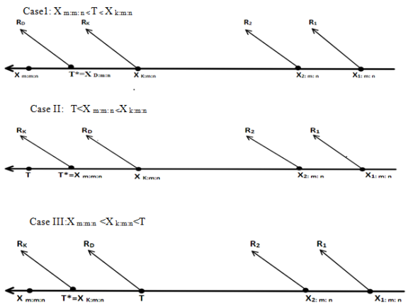
Figure 1. Schematic representation of the dual generalized progressive hybrid censoring scheme (DGPHCS).
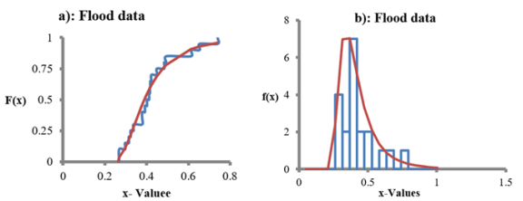
Figure 2. a) The Empirical CDF and the fitted CDF. for the flood data. b) The Histogram and the fitted PDF. for the flood data.
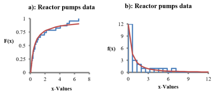
Figure 3. a) The Empirical CDF and the fitted CDF for the reactor pumps data. b) The Histogram and the fitted PDF. for the reactor pumps data.